> Complete content index: https://sondelali.com/llms.txt
# Why Your Agent Misses Answers That Are Already in Your Documents
> The rule is on page 31 of your handbook, but your agent provides a different answer. Your search engine returns whole indexed pieces of your documents, and the right size for those pieces depends on how long your documents are. In this article, I will show you how you can tell whether to cut your documents, where to cut them, and how you can prove the choice on your own questions.
URL: https://sondelali.com/blog/chunking-decides-what-you-can-find
Published: 2026-08-31
Updated: 2026-09-29
Category: Technology
 Imagine that somebody asks your agent when they can take parental leave. The rule is on page 31 of your handbook, but your agent provides a different answer. Your search engine returns other pieces of the handbook, so your agent generates its answer from those pieces.
Your search engine returns whole indexed pieces, which means that the size of each piece is a choice at the moment of loading your documents. The name for cutting long documents into smaller pieces before indexing them is **chunking**. Every cut changes which of your questions have their answer inside a single piece.
Microsoft recommends pieces of 512 tokens with an overlap of 25 per cent as the starting point for [Azure AI Search](https://learn.microsoft.com/en-us/azure/search/vector-search-how-to-chunk-documents), while [Amazon Bedrock](https://docs.aws.amazon.com/bedrock/latest/userguide/kb-chunking.html) cuts your documents into pieces of about 300 tokens by default. Three public collections of documents, each cut into pieces of several sizes and searched with the same marked questions, make up the test in this article.
Whether cutting raises the score depends on how long the documents are. On scientific abstracts and medical documents of about 200 words each, the keyword score changes by two hundredths or less in either direction between whole documents and smaller pieces. The score here is nDCG@10, which ranges from 0 up to 1.0 for a perfect ranking. On Wikipedia articles with a median of 4,675 words, however, the same score rises from 0.82 to 0.90 with pieces of 100 words, while the ten pieces that the search engine returns first hold about 1,000 words in place of about 71,000.
On the short documents, most of the change is invisible in the averages. On NFCorpus at 50 words, for example, the average score moves by less than a hundredth, while the index returns a different set of answers for 61 of the 323 questions.
In this article, I will show you how you can tell whether to cut your documents, where to cut them, and how you can prove the choice on your own questions.
## What goes wrong when the cut falls in the wrong place
The first failure is a cut straight through an answer. Take the returns policy in an online shop's help centre, where the heading 'Returns and refunds' is at the top of the section and the words 'within 14 days of delivery' appear four paragraphs below it. With a cut between those two lines, the first piece has the topic without the rule, while the second has the rule without the topic. When a customer then types a question about how long they have to send a jacket back, the search engine matches their words with the first piece on 'returns' and with the second on '14 days', which means that neither piece holds the whole answer.
Repeat the heading at the start of every piece to repair that failure, because each short piece then starts with its topic. Microsoft's authors suggest the same repair in their guidance for Azure AI Search, where the authors add the document title to the pieces from the middle of a long document.
The second failure happens when a piece is too long. In a keyword search engine, the score of a piece rises with every word of the question that appears in that piece. The score rises further for a word that appears several times, although the increase from each repeat is smaller than the increase from the one before. However, the longer a piece is than the average piece in the index, the lower its score is, because one mention of 'leave' in a section of 150 words is a stronger sign of the topic than one mention in a handbook of 12,000 words.
[Narsil](https://narsil.sondelali.com) scores keyword matches with a formula named **BM25**, which has two settings: `k1` for how far the score can rise from repeats of one word, and `b` for how far the score falls for length. At a `b` of 0, the score of a piece is the same at any length, while at 1, the fall for length is at its largest. The default for `b` in Narsil is 0.75.
Suppose that your handbook of 40 pages is one record in the index, beside a staff newsletter of 300 words with a single line about parental leave. The words 'parental leave' appear on page 31 of the handbook, where the rule is, and on several other pages as well. However, the engine can rank the newsletter above the handbook, because the fall in the handbook's score for its length is larger than the rise from its extra mentions. Once you cut the handbook at its headings, the section on parental leave becomes a short record of its own, which the engine can rank above the newsletter.
The third failure happens in vector search, because an embedding model processes only the start of a long text. According to the [model card](https://huggingface.co/sentence-transformers/all-MiniLM-L6-v2) for all-MiniLM-L6-v2, the default model in the Transformers.js adapter for Narsil, the input limit of the model is 256 tokens, and its authors train it on texts of up to 128 tokens. In my measurements, the adapter returns the same vector for a text once the text is longer than 512 tokens. The vector for a whole article of 4,675 words therefore represents only its opening.
Larger pieces or repeated headings prevent the first failure, while smaller pieces prevent the second and the third. The size that suits your documents therefore depends on how long they are.
## The scores on short and long documents
Three public test collections make up the comparison, with a list for every test query of the documents that count as relevant to it. In this article, each test query is a question, and each of its relevant documents is a marked answer. Two of the collections, both of them with short documents, come from [BEIR](https://github.com/beir-cellar/beir).
In SciFact there are 5,183 scientific abstracts with a median length of 192 words, and 300 questions with 339 marked answers between them. Each of those questions is a scientific claim, such as 'A deficiency of vitamin B12 increases blood levels of homocysteine'. In NFCorpus there are 3,633 medical documents with a median length of 224 words, and 323 questions in non-technical English from the NutritionFacts.org website. The NFCorpus authors build its 12,334 marked answers automatically from the links on that website.
The third collection, [MLDR](https://huggingface.co/datasets/Shitao/MLDR), holds long Wikipedia articles. The [MLDR authors](https://arxiv.org/abs/2402.03216) pick a paragraph at random from each article and have GPT-3.5 generate one question about that paragraph. The authors then mark the whole article as the answer to that question, although the answer is in one paragraph of that article, in the way that the parental leave rule is on one page of your handbook. The English test set has 800 questions over 200,000 articles. The sample for this test holds 5,000 of those articles: the 800 with a marked answer, and a random selection of 4,200 others from the same range of lengths. Matching the lengths matters here, because the marked articles have a median of 4,672 words against 1,440 for a random sample of the rest, while a keyword search engine scores a long document lower.
Each collection has one index of whole documents and four more indexes of pieces. The cuts for the short documents fall every 200, 100, 50, and 25 words, and the cuts for the Wikipedia articles fall every 800, 400, 200, and 100 words. Each piece is its own record in the index, under the identifier of its parent document, with the document's title at the start of the piece where the collection gives one. The BM25 settings stay at `k1` 0.9 and `b` 0.4 across every keyword index, which leaves the split as the only difference between the indexes.
Each index has two scores. The first is nDCG@10 over documents, where each piece that the engine returns counts as the document that it comes from, and each document counts once. That number measures whether the engine ranks the right documents first. The second is the share of questions for which the first ten pieces include one from a marked document, since those ten pieces are what a model receives in a prompt with the first ten results.
On the two collections of short documents, the keyword scores barely change. On SciFact, nDCG@10 is 0.6814 for whole documents and stays between 0.6613 and 0.6877 across the four splits, while on NFCorpus it is 0.3283 for whole documents and stays between 0.3190 and 0.3313. At 25 words, the first ten pieces include one from a marked document for fewer of the questions than whole documents do, at 76 per cent against 83 on SciFact and 63 per cent against 70 on NFCorpus.
A vector search engine ranks the right documents higher on the same collections at 100 words and below. On SciFact, nDCG@10 rises from 0.6550 for whole documents to 0.6908 at 25 words, and on NFCorpus it rises from 0.3126 to 0.3365. The first ten pieces, however, include one from a marked document for fewer of the questions. That share falls on SciFact from 81 per cent for whole documents to 75 per cent at 25 words, and on NFCorpus from 69 to 60 per cent, since several of the ten pieces can come from one document.
On the Wikipedia articles, the keyword score rises at every split. nDCG@10 goes from 0.8204 for whole articles to 0.8752 at 800 words and to 0.9004 at 100 words. The share of questions with a marked piece among the first ten rises from 89 to 93 per cent, while those ten pieces hold 996 words at 100 words each, against 70,944 words for ten whole articles.
Only keyword search appears in the measurements on the Wikipedia articles. For vector search, the third failure above applies to every whole article in the sample, since the adapter embeds only the first 512 tokens of each article.
[Narsil](https://narsil.sondelali.com) hosts every index in this comparison. SciFact and NFCorpus come from the same
files as Narsil's benchmark suite, while MLDR comes from the release by its authors. In every keyword index, each
record holds the title and one body piece in a single field. For every vector index, the Transformers.js adapter for
Narsil embeds each piece with all-MiniLM-L6-v2, and Narsil compares the query with every vector. For each question,
the test script retrieves the first 1,000 pieces, replaces each piece with its parent document, drops the repeats,
and keeps the first 100 documents. With every document whole, the keyword scores equal those of Narsil's benchmark
suite on 28 September 2026, at 0.6814 nDCG@10 on SciFact and a recall@100 of 0.2489 on NFCorpus.
The difference between the two groups comes from the length of the documents. A SciFact abstract has a median of 192 words, which means that each cut splits one short text across several pieces. A keyword search engine, however, matches a piece of 100 words from a Wikipedia article mainly with the questions about its own paragraph, while BM25 lowers the score of the whole article of 4,675 words for its length.
## Do this to your own documents
Measure how long your documents are first, and pick your starting point from the list below.
- For documents of a few hundred words, index each document whole. On both of the short collections, the keyword score changes by two hundredths or less between whole documents and pieces, while the first ten pieces include a marked document for fewer of the questions.
- For documents of thousands of words, cut each document at its headings, repeat each heading at the start of its pieces, and split any section that is longer than your chosen size.
- For vector search, keep every piece within the input limit on the model card of your embedding model. For all-MiniLM-L6-v2, that limit is 256 tokens, which comes to about 160 to 180 words of English in these collections.
Then compare two sizes on your own marked questions: your current size and half of it. Read the share of questions with a marked answer at the depth that goes to the model, and read it question by question.
| What you find | What to do next |
| --- | --- |
| The half-size index returns more marked answers inside the depth that goes to the model. | Halve the size again and repeat the same comparison, for as long as that share rises with each round. On the Wikipedia articles, the score rises in this way all the way down to 100 words. |
| The half-size index returns fewer of them there. | Keep the larger size, as on the short documents with keyword search. |
| The two indexes return the same marked answers. | Check your vocabulary next, because your users may be asking in words that are absent from your documents. |
With any of the three results, keep the list of individual questions, because the average may move by only about a hundredth while dozens of the questions underneath it change.
Everything that you need to act is in the steps above. The sections below hold three more things: why the average is the wrong number to trust on short documents, what researchers measure about the size of a piece, and how to make the comparison so that you can trust the result.
## Read the individual questions underneath the average
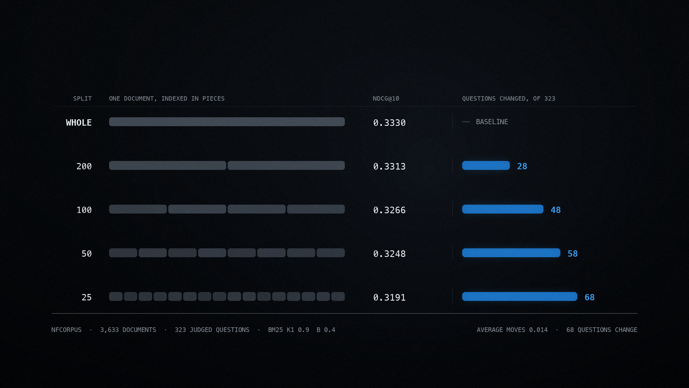
On short documents, the average is the wrong number to read, because a difference of a hundredth leads to the same decision either way. On NFCorpus, at 50 words, nDCG@10 falls from 0.3283 to 0.3254. Underneath that difference of 0.0029, the index returns more marked answers in the top ten for 25 of the 323 questions and fewer for 36, which makes 61 questions with a different result.
The same pattern appears at every split on NFCorpus. The number of questions with a different result ranges from 33 at 200 words to 82 at 25 words, while the average stays within 0.01 of the score for whole documents. A reviewer who reads only that average sees no problem at all, although at 25 words the index returns a different result for one question in four.
On the Wikipedia articles, the changes go mostly in one direction. At 100 words, the keyword search engine moves the marked article into the top ten for 41 questions and out of it for 4, while the rank of the marked article rises for 138 questions and falls for 21.
Sort your own questions by how far each of them moves, and then read both ends of that list for what the questions at each end have in common, such as an answer in a single sentence or an answer that spreads across a procedure, a table, or a numbered list. When the questions whose scores fall share a document type, give that type a splitting rule of its own, because one global setting improves one group at the expense of the other.
## Cut at the headings before you cut by size
A second comparison on the Wikipedia articles covers two ways of cutting at the same size. In the first way, a cut falls after every 200 words. In the second way, a cut falls at every section heading, any section longer than 200 words splits into pieces of up to 200 words, and every piece starts with the heading of its section. The index cut at headings scores 0.8936 against 0.8916, and at 400 words the same index scores 0.8902 against 0.8862.
With an overlap of 50 words between neighbouring pieces, which is the 25 per cent that Microsoft suggests for Azure AI Search, the score at 200 words rises from 0.8916 to 0.8957. Both of those gains are small next to the difference between whole articles, at 0.8204, and pieces of 200 words, at 0.8916.
The name for cutting where the topic changes is **semantic chunking**. Renyi Qu, Ruixuan Tu, and Forrest Bao measure it against fixed-size chunking in [Is Semantic Chunking Worth the Computational Cost?](https://arxiv.org/abs/2410.13070) (October 2024), where the authors conclude that 'the computational costs associated with semantic chunking are not justified by consistent performance gains'. In their test of document retrieval, an index of semantic chunks scores higher on documents that the authors build by joining unrelated texts together, while an index of fixed-size pieces scores higher on the original documents, at 90.59 against 87.37 on HotpotQA.
Carlo Merola and Jaspinder Singh then compare two newer techniques in [Reconstructing Context](https://arxiv.org/abs/2504.19754) (April 2025), where neither of the two comes out ahead on every measure. The two authors report that contextual retrieval preserves semantic coherence more effectively at a higher computational cost, and that late chunking works more efficiently at some loss of relevance and completeness.
## Match the size of a piece to the questions that people ask
Sinchana Ramakanth Bhat and colleagues test fixed-size chunking with vector search on long documents in [a May 2025 multi-dataset analysis](https://arxiv.org/abs/2505.21700). The authors find that chunks of 64 to 128 tokens score best on the datasets whose answers are short facts, while chunks of 512 to 1,024 tokens score best where the answer spans a broader passage. With the Stella embedding model, recall@1 on TechQA rises from 4.9 per cent at 64 tokens to 61.9 per cent at 1,024 tokens, while on SQuAD it falls from 64.2 to 38.6 per cent across the same range. The same authors find that the best size differs from one embedding model to the next, so a change of model means a new decision about size.
Each MLDR question comes from one paragraph, and the answer to it is therefore in a short passage. On those articles, the keyword score rises all the way down to 100 words, the smallest size in this test, which fits what Bhat and colleagues find for short answers.
A search engine ranks a small piece well, although the answer to a question can span the text around that piece. Amazon provides **hierarchical chunking** in Bedrock for that case, where the search engine matches small child pieces and then replaces each of them with its larger parent piece before the model receives the results. On the Wikipedia articles, ten pieces of 100 words hold about 1,000 words, which leaves room in the prompt for the section around each of them. The measurements here cover the ranking alone, not the answers that a model generates from those pieces.
A published size is the result of somebody else's careful measurement on their own documents. Use it as the
starting point for your own comparison, and measure it on your documents before you adopt it.
## Making the comparison so that you can trust the answer
A comparison of this kind rests on a set of real questions with the right documents marked for each one, which is the judged set from [the previous article](/blog/prove-your-retrieval-works). Keep every other setting where it is.
Use the same questions and the same relevance marks for every index. Adding a question between the indexes, or
revising a mark after one index scores better with it, makes the comparison meaningless.
Load the identical source files into every index, and change only where the cuts fall. Start from your current
size, and then add one index at half that size and one at double it, since one step in each direction is enough to
tell which way to go.
Keep the analyser, the language, `k1`, `b`, the retrieval mode, and the number of results identical across every
index. A change to the splitting and the ranking together leaves no way to attribute the result to either one.
If your application sends ten passages to the model, recall at ten is the number to read, because recall at ten
measures the share of marked answers inside the set that the model receives.
With whole documents as the unit, as in this article, the marks stay the same for every index, since each piece
maps back to a document with a mark already. With pieces as the unit, each new split produces pieces that are
unmarked, while `trec_eval` scores an unmarked piece as irrelevant. In that case, pool the new candidates,
grade them under your existing grading rule, and only then compare.
When the index for one split scores higher on your judged set, that higher score holds for the questions in that set
so far. Repeat the comparison when the shape of your documents changes, or when your users start bringing a kind of
question that is not yet in your judged set.
## When the split makes no difference either way
When the split makes no difference either way, the next thing to check is the vocabulary in your documents. A keyword search engine matches those words, which is why the engine returns nothing for 'time off for a new baby' from a handbook whose wording is 'parental leave' throughout, at any piece size. That vocabulary gap is the second limit in this study. In [the next article](/blog/is-vector-search-worth-it), I will show you how you can tell what vector search can find, what you pay for it, and whether it is worth that for you.
## Updates
### 17 September 2026
**[The scores on short and long documents](https://sondelali.com/blog/chunking-decides-what-you-can-find#the-scores-on-short-and-long-documents)**
In the version of 31 August 2026, I write that researchers mark the answers in both collections, and I call the NFCorpus documents nutrition articles. In the version of 17 September 2026, I say that the NFCorpus authors build their marks automatically, that the documents are medical documents, and that each SciFact question is a scientific claim.
### 28 September 2026
**[What goes wrong when the cut falls in the wrong place](https://sondelali.com/blog/chunking-decides-what-you-can-find#what-goes-wrong-when-the-cut-falls-in-the-wrong-place)**
In the version of 31 August 2026, I describe two failures. I now add a third failure for vector search, along with the repeated heading as the repair for the first.
**[The scores on short and long documents](https://sondelali.com/blog/chunking-decides-what-you-can-find#the-scores-on-short-and-long-documents)**
In the version of 31 August 2026, I measure SciFact and NFCorpus at five splits each with Narsil 0.2.2, and I write that nDCG@10 falls at every smaller size, from 0.6757 to 0.6309 on SciFact and from 0.3330 to 0.3191 on NFCorpus. I now measure with Narsil 0.3.0, and I add vector search and a sample of 5,000 long Wikipedia articles from MLDR. On the short documents, the keyword score stays within two hundredths of the score for whole documents, while on the Wikipedia articles it rises from 0.8204 to 0.9004 at 100 words.
**[Do this to your own documents](https://sondelali.com/blog/chunking-decides-what-you-can-find#do-this-to-your-own-documents)**
In the version of 31 August 2026, I tell you to compare your current size with half of it, and to leave the splitting as it is when the smaller pieces score lower, which is the result that I report on both corpora. I now tell you to index short documents whole, to cut long documents at their headings, and to keep every piece within the input limit of your embedding model before you compare two sizes.
**[Read the individual questions underneath the average](https://sondelali.com/blog/chunking-decides-what-you-can-find#read-the-individual-questions-underneath-the-average)**
In the version of 31 August 2026, I write that on NFCorpus at 50 words the average falls from 0.3330 to 0.3248 while 58 questions change. With Narsil 0.3.0, the average falls from 0.3283 to 0.3254 while 61 questions change, and I add the figures for the Wikipedia articles.
**[Match the size of a piece to the questions that people ask](https://sondelali.com/blog/chunking-decides-what-you-can-find#match-the-size-of-a-piece-to-the-questions-that-people-ask)**
In the version of 31 August 2026, I report the size ranges from Bhat and colleagues without their figures. I now give their recall figures for TechQA and SQuAD, my figures for the Wikipedia articles, and hierarchical chunking in Amazon Bedrock.
**[Making the comparison so that you can trust the answer](https://sondelali.com/blog/chunking-decides-what-you-can-find#making-the-comparison-so-that-you-can-trust-the-answer)**
In the version of 31 August 2026, I tell you in the last step to judge the new candidates from each split. I now write that this step applies when you score the pieces themselves, since you keep the same marks for every index when you score whole documents.
### 29 September 2026
**[What goes wrong when the cut falls in the wrong place](https://sondelali.com/blog/chunking-decides-what-you-can-find#what-goes-wrong-when-the-cut-falls-in-the-wrong-place)**
In the version of 28 September 2026, I write that the adapter returns the same vector once a text is longer than 512 word pieces. I now add the input limit of 256 tokens from the model card for all-MiniLM-L6-v2.
**[Do this to your own documents](https://sondelali.com/blog/chunking-decides-what-you-can-find#do-this-to-your-own-documents)**
In the version of 28 September 2026, I tell you to keep every piece for vector search within 512 word pieces for the model in this test. I now tell you to keep it within the input limit on the model card, which is 256 tokens for all-MiniLM-L6-v2, or about 160 to 180 words of English in these collections.